The 3 Dimensions they didn’t tell you about

Dimensional Analysis Revisited

These aren’t your ‘tiny curled up extra dimensions of space’.

Loads of media covering that kind of stuff.

I am referring to Mass, Length and Time.

Feel cheated, don’t you ?

But so did the Americans, when it was exactly these quantities that exposed their most closely guarded military secret.

Want to know how ?

What is a Dimension ?

Dimension is a curious thing.

The term is used differently in different situations. But, in the context of physical quantities, dimension is just a label used to determime commensurability.

Commensurable quantities are quantities of the same kind. Such as kilometres and miles. Both tell us something about the distance, displacement, length, width or maybe even height.

But, why do we care about commensurability ?

Because, only commensurable quantities are comparable.

We choose a convenient set of base dimensions of quantity such that every physical quantity can be expressed in terms of elements of this set (which are dimensions).

The traditional base dimensions are mass, length, time, charge, and temperature.

In principle, however, other base quantities could also have been used. For instance, the International System of Units (SI) considers seven base units - kilogram (mass), metre (length), candela (luminous intensity), second (time), ampere (electric current), kelvin (temperature), and mole (quantity).

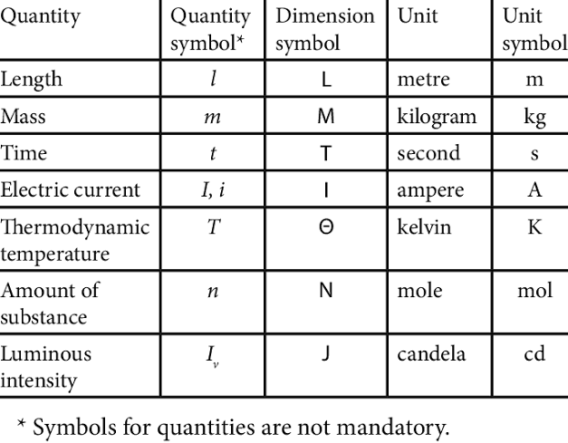
SI base units, dimensions and their symbols

(Source : https://www.researchgate.net/figure/SI-base-quantities-and-units-and-their-symbols_tbl1_341161233)

As mentioned before, here electric current has been used instead of charge. Along with these base units, several derived units have also been defined.

Many have special names and symbols as a tribute to researchers.

Homogeneity of Units

Even before the notion of dimensions was made concrete, researchers knew that adding length to an area doesn’t make any sense.

This idea is captured by the principle of homogeneity.

The principle of homogeneity states that if A = B is physically meaningful, then A must have the same units as B.

Similarly, if A + B appears in an equation, then A must have the same units as B.

Euclid

Euclid’s Elements contains an early statement of this principle.

It states that ‘only things of the same kind can be compared to each other, where angles, lengths, areas and volumes are the different kinds. Greek mathematics was entirely based on geometry, and arithmetic expressions were considered to be sums and products of lengths and areas.

So, everything had a geometrical interpretation.

Descartes (1596–1650)

Development of analytical geometry broke this Greek tradition.

Descartes considered curves in the plane described by equations such as y = x²+x³, where he assumed that x and y were lengths. To justify these equations, the French polymath stated that the higher-order terms (such as x² and x³) are implicitly multiplied by some power of the unit length u.

So, the equation actually read y = x²/u+x³/u², giving all terms the dimension of length. This means that analytic geometry requires a reference length (the unit length).

Whereas Euclidean geometry was devoid of any such preferred length.

Doing Physics without reference to Dimensions of Quantities

Galileo (1564–1642)

Galileo’s Two New Sciences describes trajectories and times of flight of objects moving without air resistance.

In it, he speaks of the ‘speed’ of particles, but his results are stated in terms of ratios of distances and times.

For instance,

‘If two particles are carried with uniform motion, but each with a different speed, the distances covered by them during unequal intervals of time bear to each other the compound ratio of the speeds and time intervals.’

(Proposition IV, Third Day, Galileo’s Discourse concerning Two New Sciences)

Galileo thought it was not sensible to take the product of a speed, or velocity and a time, as we do in the modern statement of this proposition: d = vt.

So, he never spoke of the numerical values of speeds and only ever referred to the ratios of speeds.

Newton

We see this with Newton as well.

In his Principia Mathematica, speaking of forces and other dimensioned quantities, Newton treats forces as Galileo treated velocities. That is, he acknowledged that force has a physical meaning and talked about ratios of forces. But he refrained from commenting on the numerical value of a force.

So, he never wrote an equation where force appears alone on one side.

For instance, in the section of the Principia on the contribution of the Sun and moon to tides, Newton writes,

‘Wherefore since the force of the Sun is tothe force of gravity as 1 to 12 868 200, the Moon’s force will be to the force of gravityas 1 to 2981 400’

(Proposition XXXVII, Problem XVIII, Book 3)

The LHS as well the RHS are just some number without any dimensional value.

Talking about ratios of quantities eliminated the use of dimensions altogether.

Birth of Dimensions

Fourier (1768–1830)

A novel thought struck Joseph Fourier.

He felt that the laws of nature, and the fundamental equations we use to describe them should be independent of the systems of units employed to measure the physical variables. That is, they should be equally valid in the Metric System of units, as in a non-metric system of units.

So, when converting between these two systems of units, we needed to be aware only of the mathematical factors required to convert between their base units.

In that light, the 19th century Mathematician seems to be the first to recognize that physical quantities have units associated with them. These units (of dimensions) determined how these quantities rescale under changes in the system of units employed to quantify them.

Fourier was also one of the first to explicitly state that physical quantities have dimensions :

‘In order to measure these quantities and express them numerically, they must be compared with different kinds of units, five in number, namely, the unit of length, the unit of time, that of temperature, that of weight, and finally the unit which serves to measure quantities of heat.’

Chapter : General Remarks - The Analytic Theory of Heat (Section IX)

Fourier’s Dimensional Analysis

Fourier’s calculations involve three coefficients, namely thermal transmittance (K), thermal conductance (h) and heat capacity (C).

These differ between materials and have a non-trivial dependence on modern fundamental units. He realized that these constants must rescale when we change the system of measurement units. Fourier also pointed out that this rescaling factor must depend on the exponent of the dimension involved in the property of interest.

For example, an area and a volume have exponents of dimension 2 and 3 (that is, L² and L³, respectively) with respect to the dimension of length.

The Specific heat (C), which is the heat required to raise the temperature of a volume of a material by one degree, has exponent of dimension −3 with respect to length.

So, if the unit of length is divided by λ, then the numerical value of C is multiplied by λ³.

Fourier provided a table specifying the dimensions of the undetermined constants k, h and C.

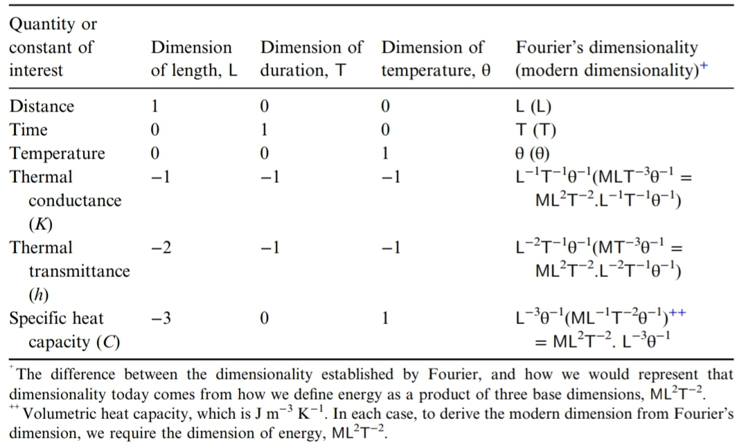
Fourier’s dimensional analysis of some properties of solid

(Source : Dimensional Analysis : The great principle of similitude by Jeffery H Williams)

This led Fourier to a generalized principle of dimensional homogeneity, which applies to linear equations and differential equations :

‘On applying the preceding rule to the different equations and their transformations, it will be found that they are homogenous with respect to each kind of unit, and that the dimension of every angular or exponential quantity is nothing.’

Consequently, just as we cannot add a length to an area, we also cannot add quantities A and B, if A has units of second (s) and B has units of second squared (s²).

Fourier’s insights on dimensional analysis far surpassed those of anyone who preceded him.

Yet, he did not realize the full potential of this insight.

The method of using dimensions of the quantities involved to infer the form of the equation relating them would only be first used in the late 1800s by Lord Rayleigh.

Dimensional Arguments

Rayleigh Algorithm

Lord Rayleigh pioneered the use of dimensional arguments in physics.

He used them extensively in his Theory of Sound (1877), which contained a section entitled, Method of Dimensions.

Following example demonstrates its usage in a simple problem :

Suppose we are interested in finding the frequency (f) of the small oscillations made by a mass (m) attached to one end of a massless spring of spring constant (k), the other being fixed to a rigid wall.

f, we believe, is a function of m, k and A.

But, we don’t know the particulars of the exact relations beforehand.

So, we assume the unknown quantity f to be proportional to some function containing the variables known to be involved in the problem.

That is,

where C is an unknown constant of proportionality.

The dimensions of these quantities are as follows :

[m] = M¹L⁰T⁰

[k] = M¹L⁰T-²

[A] = M⁰L¹T⁰

Where M, L, T are mass, length and time respectively.

Evidently, g(m, k, A) must have dimension T^(−1). Lord Rayleigh argued that the relation, f = g(m, k, A) should hold regardless of the choice of units.

Thus, both sides must rescale in the same way when we change units.

To do this, we must find a, b and c such that

This gives us a set of linear equations (one for each base dimension) that must be solved.

The unique solution: a = −1/2, b = 1/2 and c = 0 implies

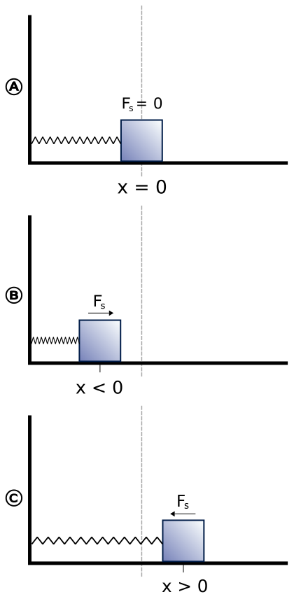
The frequency (f) of the spring-mass system depends only on the spring constant (k) and the mass (m)

(Source : https://en.m.wikipedia.org/wiki/Harmonic_oscillator)

A limitation of dimensional analysis is its inability to cannot comment on this constant C.

However, such non-dimensional constants are usually determined experimentally. So they are beyond the scope of theoretical considerations anyways. For this specific problem however, an exact formula does exist. It is 2πf = √(k/m).

This technique of equating exponents of dimension is called the Rayleigh algorithm.

Rigorous Formulation

In the 1880s and 1890s, French scientists began to develop a more general and rigorous theory of dimensional analysis.

Aimé Vaschy (1857–1899) wrote in 1896:

‘Any homogenous relationship among p quantities a1, a2, …, ap, the values of which depend on the choice of the units, may be reduced to a relationship involving (p-k) parameters that are monomial combinations of a1, a2, …, ap and that are of zero dimensions.’

Vaschy’s theorem was soon forgotten.

However, it was rediscovered independently by Dimitri Pavlovitch Riabouchinsky (1882–1962) in Russia in 1911 and by the American Edgar Buckingham (1867–1940).

The latter went on to write a series of papers on the subject in 1914, citing both Riabouchinsky and Vaschy.

The modern form of this theorem, concerning the number of coupled variables in a phenomenon is now commonly called the Buckingham Π-theorem.

It is named so because of the use of the Greek letter Π as a label for the groups of dimensionless variables.

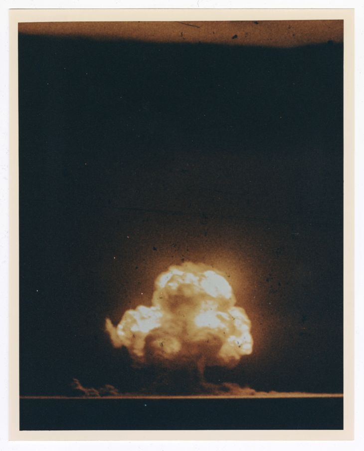
GI Taylor Incident

Trinity was the code name of the first detonation of a nuclear weapon a as part of the Manhattan Project.

The British mathematician, Sir G.I. Taylor was present at the Trinity nuclear test, July 16, 1945, as part of General Leslie Groves’ “VIP List” of 10 people who observed the test from Compania Hill, about 20 miles (32 km) northwest of the shot tower. Based on his knowledge of fluid dynamics and conventional explosions, he published a report for the Ministry of Home Security.

In this report, he attempted to determine the expected effects of such nuclear explosions.

Only color photo of the first atomic detonation at the Trinity Site, 1945

(Source : https://nmsu.contentdm.oclc.org/digital/collection/wsmr_photos/id/31/)

After the war the report was declassified and published.

Taylor’s Argument

Firstly, two assumptions need to be made :

1. The energy (E) was released in a small space.

2. The shock wave was spherical.

We have the size of the fire ball (R as a function of t) at several different times. How does the radius(R) depend on:

• energy (E)

• time (t)

• density of the surrounding medium (ρ – initial density of air)

Dimensions of the given quantities :

[p] refers to the dimensions of the quantity

• [R] = L
• [E] = ML²/T²
• [t] = T
• [ρ] = M/L³

Suppose

Then

This gives us a linear system of equations

which, upon solving gives x=1/5, y=-1/5, z=2/5.

The radius of the shock wave is therefore

What is ‘S’ ?

According to Taylor’s notation, S is a dimensionless proportionality constant.

But, unlike the constant C we saw in the dimensional argument for determining the frequency of a harmonic oscillator, S need not be a single value for all radii and times. Given the extreme conditions inside the fireball, S could change depending on which processes dominate at a particular time.

To test the validity of this equation, the radius of the fireball must be plotted as a function of time.

While plotting, linear graphs are preferred. So, the equation obtained for R is linearised by taking the common logarithm (base-10) of both sides :

Comparing the given equation with the equation of a straight line y = mx+c, we expect the slope of log R vs log t graph to be 2/5

And the intercept on y-axis (c) to be :

This is essentially the analysis Taylor performed in his second paper using declassified high-speed photos of the expanding Trinity fireball.

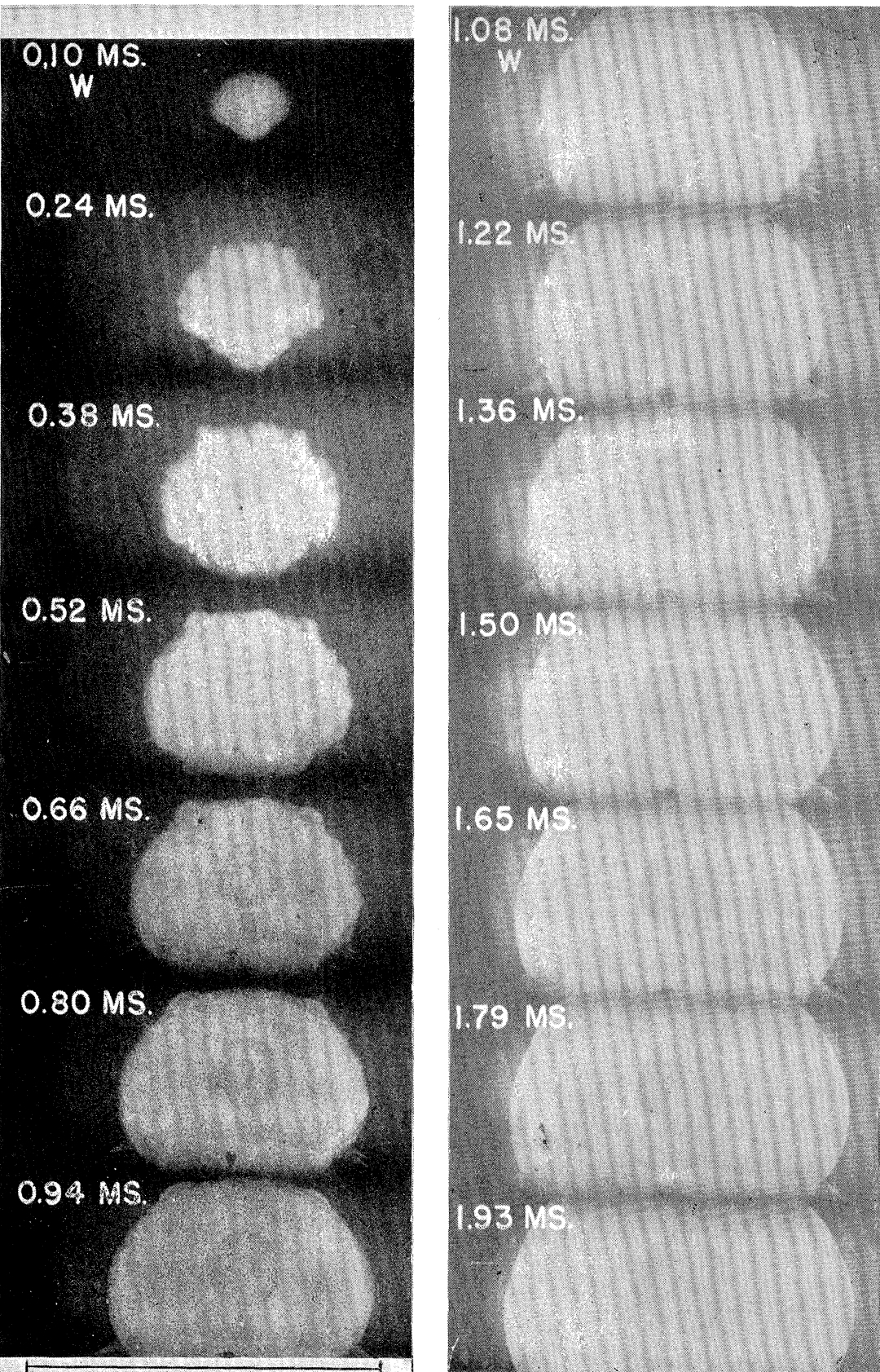
The expanding Trinity fireball captured in a series of photographs 0.1 msto 1.93 ms after detonation

The length and time scales provided on the frames allowed Taylor to accurately measure the radius of the fireball at each instant and produce the graph shown below.

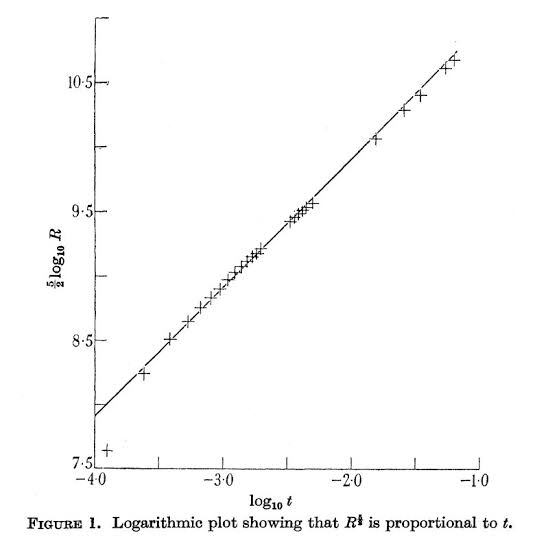
Plot of the Trinity fireball radius as a function of time, using measurements from Taylor

(Source : https://thatsmaths.com/2014/09/18/how-big-was-the-bomb/)

The agreement between the predicted slope and the measurements is remarkable given the complex physics taking place inside the fireball during this time. Only the first data point (0.10 ms after detonation when the radius was 11 m) lies significantly off the linear trend.

The initial interaction of the rapidly expanding blast wave with the bomb casing and tower presumably contributed to the deviation.

Dependence on γ

Taylor assumed S to be a function of γ, the adiabatic constant for the surrounding air.

Adiabatic constant characterises the expansion of an ideal gas in an idealized thermodynamical process (isentropic expansion), that assumes thermodynamic equilibrium of the gas with its surroundings during the entire process without involving heat transfer.

The excellent agreement between theory and measurement also implies that the explosion can be characterised by a single value of S over a wide range of times.

He notes in his second paper,

“this is surprising, because in those calculations it was assumed that air behaves as though γ, the ratio of the specific heats, is constant at all temperatures, an assumption which is certainly not true.”

Estimation of Yield

Obviously, dimensional analysis cannot provide a value for S(γ).

Since the explosion energy E depends on S to the fifth power, Taylor spent considerable effort determining its theoretical value.

For dry air at standard temperatures, γ = 1.4, so he found S(1.4) = 1.032.

Using this value and assuming an air density of 1.25 kg m–3, Taylor estimated the Trinity test to have an explosion energy of 71.4 TJ, or equivalent to 16,800 tons (16.8 kt) of TNT3. The official yield as determined by the US Department of Energy is 21 kt.

The reported yield, however, includes the mechanical energy of the blast calculated, as well as contributions from the light output and ionizing radiation.

Aftermath

A small confession.

Taylor’s approach for finding the formula and estimating the yield was much more rigorous than vanilla dimensional analysis.

They involved simultaneously solving the equation of motion, continuity equation and equation of state for an expanding spherical blast wave from a point source.

This calculation of energy caused, in Taylor’s own words, ‘much embarrassment’ in US government circles.

This was because the number was then still classified despite the photographs published by Mack being publicy available. Perhaps, Taylor was even mildly admonished by the US Army for publishing his deductions from their (unclassified) photographs.

However, the mere prospect serves the point of illustrating the sheer power of this incredible tool.

References

• Dimensional Analysis : The great principle of similitude by Jeffery H Williams
• Using dimensional analysis to estimate the yield of the Trinity nuclear test of July 16, 1945 by Simon Murphy, UNSW Canberra
• https://en.m.wikipedia.org/wiki/Taylor%E2%80%93von_Neumann%E2%80%93Sedov_blast_wave
• https://en.m.wikipedia.org/wiki/Base_unit_of_measurement